Introduction
Seemingly straightforward tasks like planting flowers can benefit from a touch of optimization (using Dynamic Programming), and provide us with new insights (and vaulable life lessons). This can be seen from the problem Can Place Flowers on leetcode.
Note : This blogpost is a follow-up of my previous blogpost - Optimizing Algorithms: From Brute Force to Beautiful. Do read it first for better understanding.
The problem
This is a problem from leetcode, Can Place Flowers.
The problem states that you have a long flowerbed in which some of the plots are planted, and some are not. However, flowers cannot be planted in adjacent plots.
Given an integer array flowerbed containing 0's and 1's, where 0 means empty and 1 means not empty, and an integer n, return true if n new flowers can be planted in the flowerbed without violating the no-adjacent-flowers rule and false otherwise.
Approach
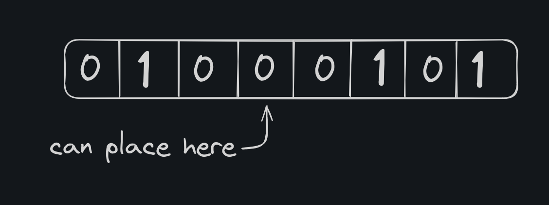
We can place a flower only when we have no adjacent flowers. So, we need a 0 in left side and right side and a 0 to place the flower itself.
A flower can be placed if there are three consecutive zeroes.
that simple ? No
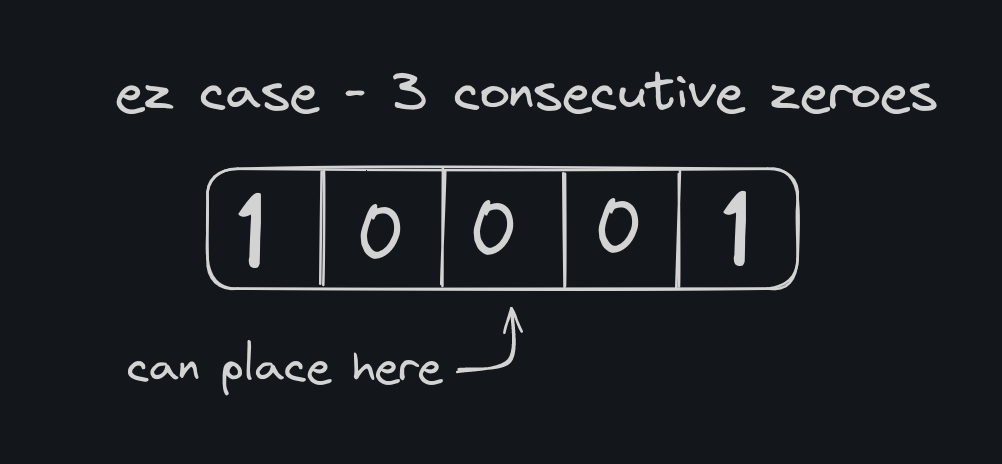
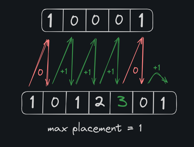
Consider the case [ 1 0 0 0 1 ], we can place 1 flower in it.
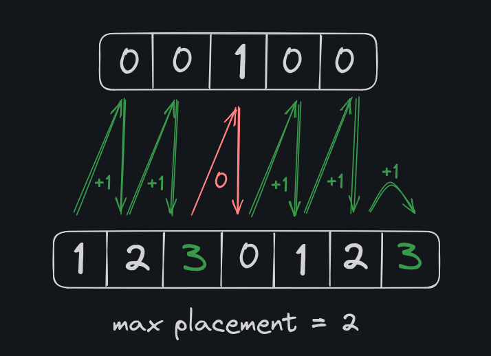
Now consider this case [ 0 0 1 0 0 ]
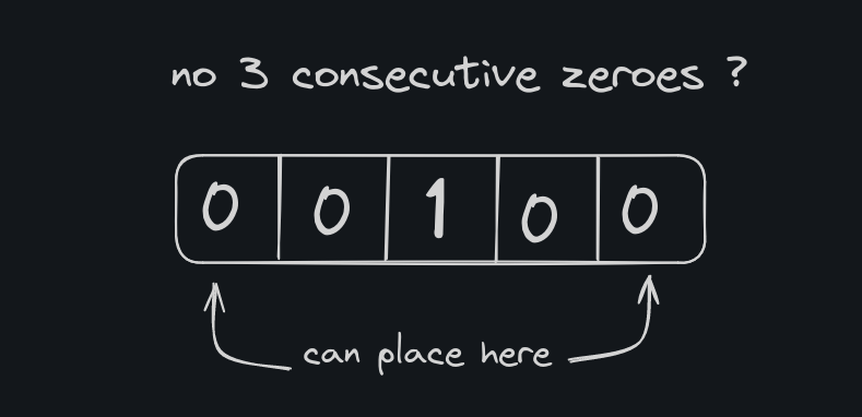
We can plant two flowers here, but there are no consecutive 3 zeroes. To tackle this we add a trailing and leading zero for all cases (atlest consider it).
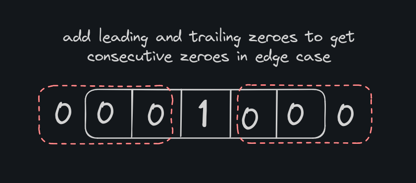
Now the array can be viewed as [ 0 0 0 1 0 0 0 ], so we can place 2 flowers max.
done ? Not yet.
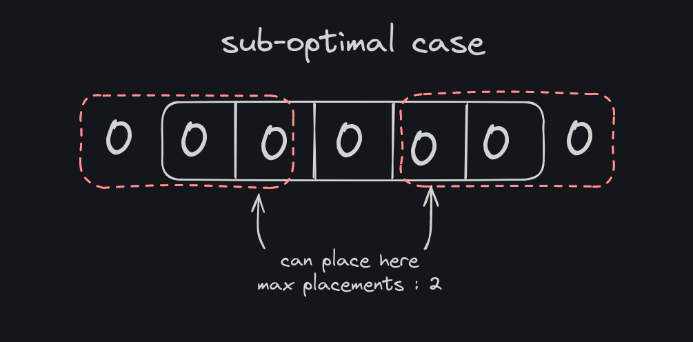
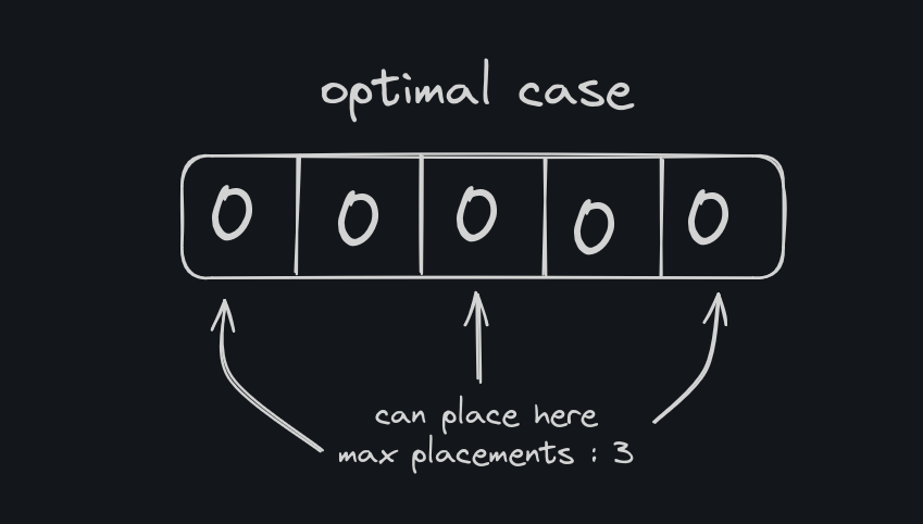
Consider this case [ 0 0 0 0 0 ]. We can plant 3 plants here, ie. [plant,0,plant,0,plant] but going by our inititution even after applying the leading and trailing zeroes, we get [ 0 0 0 0 0 0 0 ], by which we get only two pairs of leading zeroes.
So how do we solve it ? This is were DP comes in handy.
DP - Approach
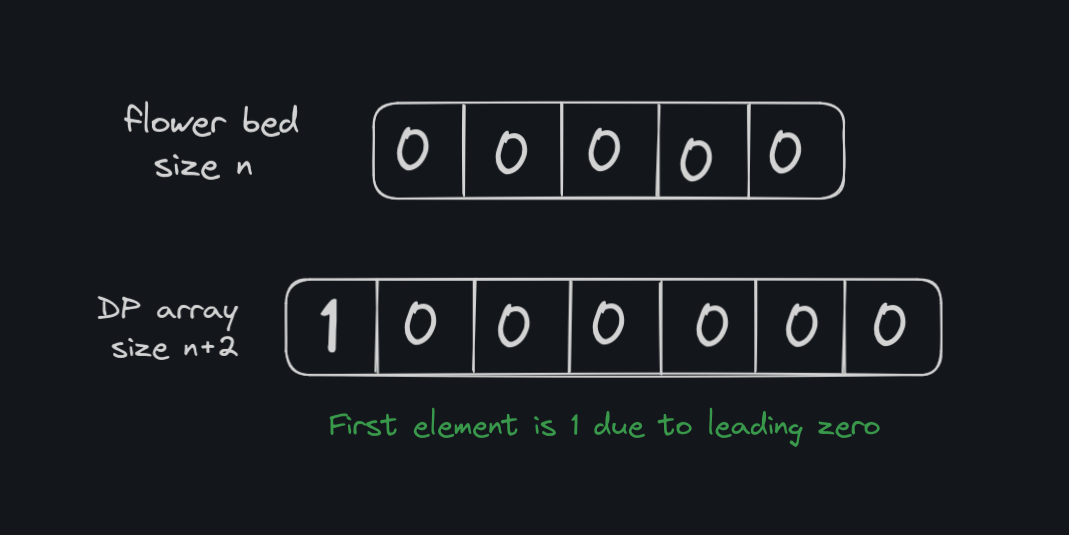
Create a dp array of length n+2 where n is the length of flowerbed.
We set dp[0]=1 as due to the leading zero.
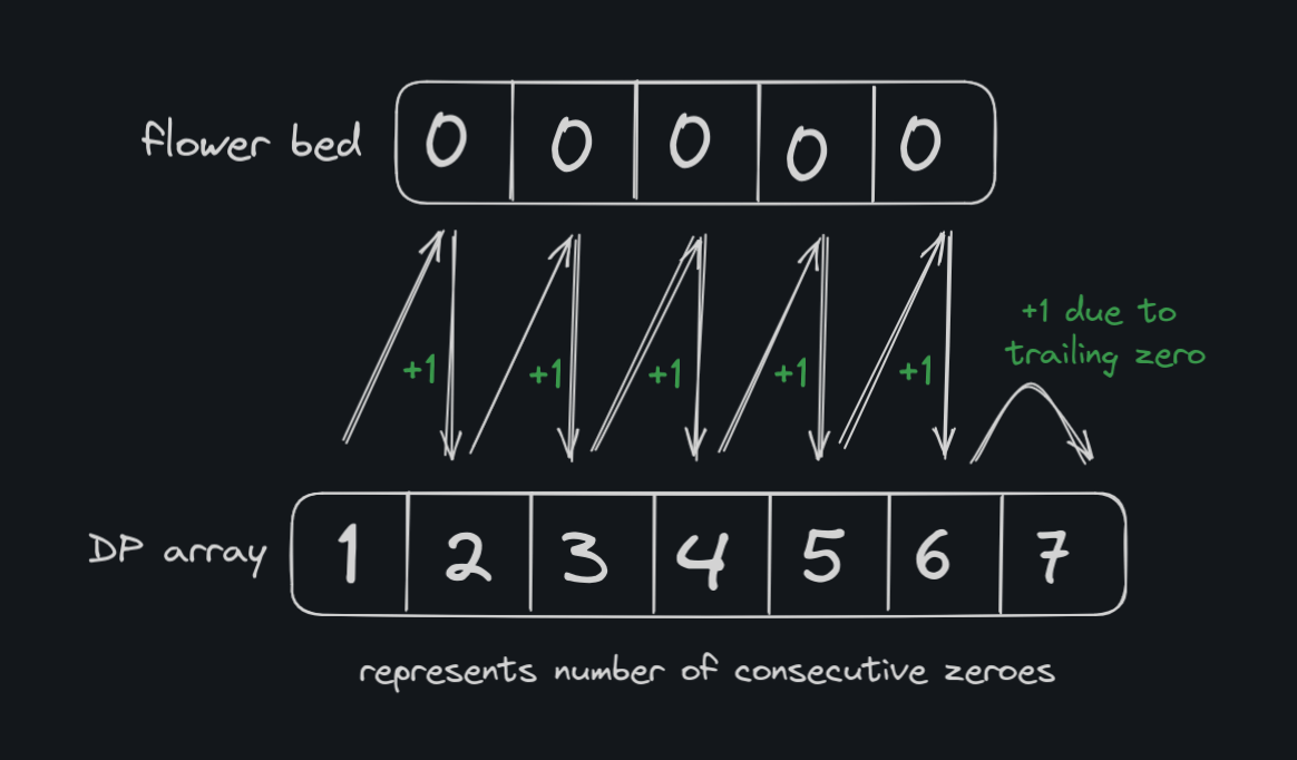
Each element in dp represents the number of continous zeroes.
now we iterate over the flowerbed, and if the flowerbed has continous zeroes, we keep adding to dp else reset it.
if(flowerbed[i]==0)
    dp[i+1] = dp[i]+1;
else
    dp[i+1] = 0;
But there's a catch. You will know it later
consider the flowerbed [ 0 0 0 0 0 ],
adding leading and trailing zeroes [ 0 0 0 0 0 0 0 ]
the continous zeroes would look like : [ 1 2 3 4 5 6 7 ]
Minor Tweaking
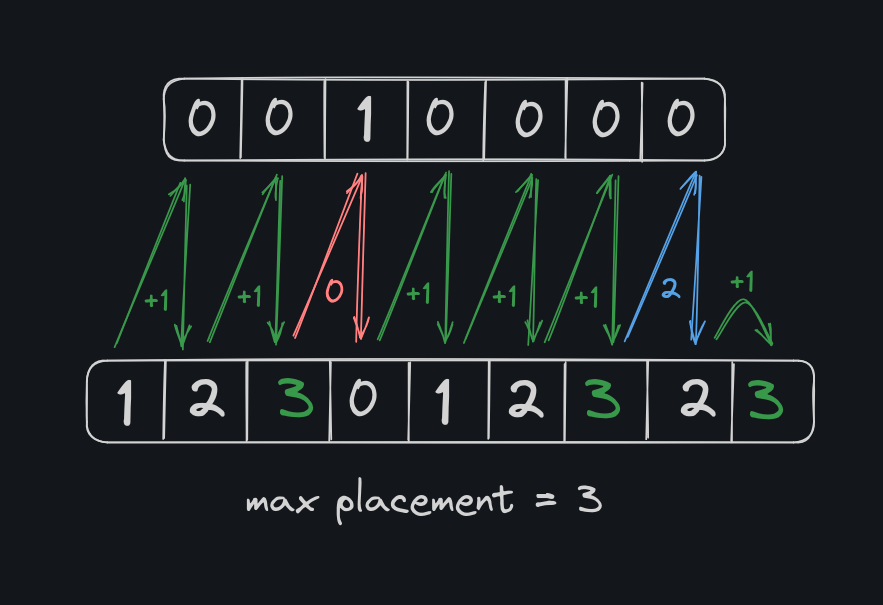
Whenever we encounter more than 3 continous zeroes, ie. if we encounter a fourth continous zero, we place it in the dp array as 2 instead of 4. (you will understand why in the end).
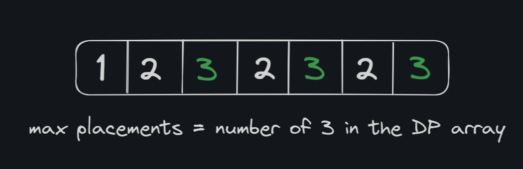
we get [ 1 2 3 2 3 2 3 ]
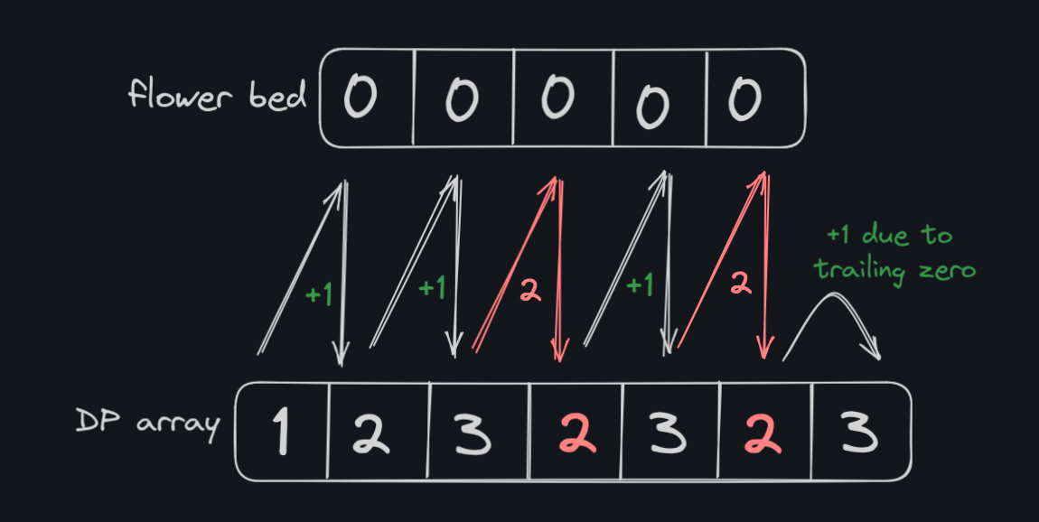
We can get the maximum number of flowers that can be placed by simply counting the number of 3's in the DP array.
Therefore we can return the boolean value of given
n <= number of 3's in the dp array
Why use 2 instead of 4 ?
If you still have not understood why we use 2 in place of 4 in the dp array, this would clear your doubt.
When we encounter four consecutive empty spots in the flowerbed, our initial instinct might be to count them as a single group of four and assume we can plant two flowers within that group. However, upon closer examination, we realize that this approach overlooks a crucial possibility.
Imagine the scenario where we have four consecutive empty spots followed by another empty spot. If the next element after those four spots is also empty, it means we can actually plant a flower in the middle of those four spots and another flower in the spot after them, without violating the rule of no adjacent flowers.
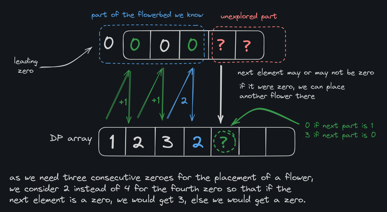
By counting those four consecutive empty spots as two pairs of two, we acknowledge the potential for planting flowers in between them and in the spot immediately after them. This adjustment ensures that our algorithm remains flexible and accurately reflects the available planting space.
Therefore, when we encounter a fourth consecutive empty spot, we replace it with a count of 2 instead of 4. This decision allows us to make more informed choices about where we can plant flowers while maintaining the no-adjacent-flowers rule. (beautiful isn't it)
This works for all cases. Let us consider our initial cases as examples
Code
class Solution {
public:
    bool canPlaceFlowers(vector<int>& flowerbed, int n) {
        vector<int> dp(flowerbed.size() + 2, 0);
        int k = 0;

        // leading zero
        dp[0] = 1;

        for (int i = 0; i < flowerbed.size(); i++) {
            if (flowerbed[i] == 0) {
                // fourth consecutive zero - change to 2
                if (dp[i] == 3) {
                    dp[i + 1] = 2;
                } else {
                    dp[i + 1] = dp[i] + 1;
                }
            } else {
                dp[i + 1] = 0;
            }
        }
        // trailing zero
        dp[dp.size() - 1] = dp[dp.size() - 2] + 1;

        for (int i : dp) {
            if (i == 3) {
                k++;
            }
        }
        return k >= n;
    }
};
Time Complexity : O(n)
Space Complexity : O(n)
Results
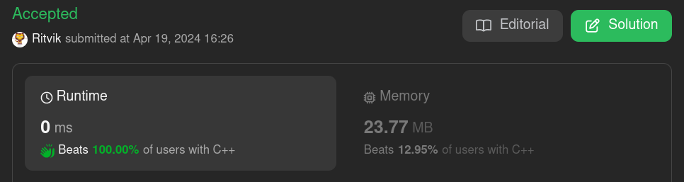
Yep, you saw it right, runtime - zero milliseconds. Although we have sacrificed a little bit of memory for this, there is always a tradeoff between time and space. We could have used a greedy algorithm without sacrificing memory, but the tradeoff would have been done with time, which may not achieve what we have achieved with the runtime.
Conclusion
The Can Place Flowers problem has shown us that even small tasks can reveal big challenges. By using dynamic programming, we found a smart way to decide where to plant flowers without breaking any rules.
We learned that sometimes, the best solution comes from thinking about the problem in a new way. Instead of just counting empty spots, we thought about how we could use them to our advantage. (preach)
This journey reminds us that in the world of algorithms, there's always more than one way to solve a problem. With a little creativity and a lot of patience, we can turn even the simplest task into an opportunity for smart thinking and clever solutions.
Optimization is not just finding solutions, but finding elegant solutions that make the most of what we have.